Back when I was a boy I was obsessed with telescopes, astronomy, and space. I saved my money and bought a three inch Newtonian reflector telescope from Edmund Scientific[1] and subscribed to “Sky and Telescope” magazine. In 1979 the Voyager 1 probe reached Jupiter and I was enthralled with the color pictures produced by the Jet Propulsion Laboratory. I understood that they were created from multiple monochrome images taken with different color filters and I wanted to do that myself.
Computers were not common back then. The high school I went to in the late 1970’s had an HP time-share BASIC computer that replaced my telescope in my affections.[2] There was no way to do real image processing on it but I wrote some simulations, one of which I’m about to describe.
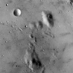
Fast-forward to 1993. The raw Voyager imagery was released on those new-fangled optical CD disks so I bought a set and an external CD-ROM drive to attach to my Dell NL25 notebook computer.[3] The JPL kindly sent me the Voyager camera and filter specifications and I finally wrote a program to create my own color composite images. One of them is this article’s featured image.
Yes, image processing is one of my hobbies but I swear I can give it up any time I want.
Recently I was doing some research on data compression when I realized that it could be used to enhance image contrast in a specific “optimal” fashion. This is actually something I’d been thinking about for some time. I implemented it and during testing made a discovery that prompted me to write this article.
The classic image contrast enhancement algorithm is called Histogram Equalization:
https://en.wikipedia.org/wiki/Histogram_equalization
Once you scroll past the math the Wikipedia article has some example images. Here’s how it works in my own words:
OCCULAR HEALTH WARNING! If your eyes glaze over at computer algorithm descriptions then just skip down to the pretty pictures.
Start with a monochrome image. Each pixel has a value ranging from zero for black to 255 for white. These are “grayscale levels”. The first step is to create census or histogram of each grayscale level. If the image is a tiny 3×3 like this:
118 120 119
120 122 121
121 120 119
Then the census array isn’t going to use the full zero to 255 grayscale range because the grayscale levels are only from 118 to 122. The census is:
[0] = 0
...
[117] = 0
[118] = 1
[119] = 2
[120] = 3
[121] = 2
[122] = 1
[123] = 0
...
[255] = 0
The next step is to create a cumulative census array by adding the census values in sequence. Census values [0] through [117] are zero so the cumulative sums for those values are zero. The first non-zero cumulative value is [118] which is one. The next cumulative value is [119] which is [119] plus [118] or three. The next is [120] which is [120] plus [119] plus [118] or six. The complete cumulative array is:
[0] = 0
...
[117] = 0
[118] = 1
[119] = 3
[120] = 6
[121] = 8
[122] = 9
[123] = 9
...
[255] = 9
Because census values [123] through [255] are zero the cumulative census values for those grayscale values remain nine.
And now for some math.[4] The cumulative range is the cumulative value of [0] to the cumulative value of [255] which is zero to nine. We need to transform this to the grayscale range of zero to 255. This is accomplished by multiplying each cumulative value by 255/9 or 28.33.[5] Since we’re using integers no decimal places are allowed so the resulting values are rounded to the nearest integer. The resulting transformed cumulative array is:
[0] = 0
...
[117] = 0
[118] = 28
[119] = 85
[120] = 170
[121] = 227
[122] = 255
[123] = 255
...
[255] = 255
The image pixel values are then changed by replacing them with the transformed cumulative value. Pixel values of 118 are replaced with [118] or 28. Pixel values of 119 are replaced with [119] or 85, etc. The resulting 3×3 image is:
 28 170  85
170 255 227
227 170  85
The original image has almost no contrast. The grayscale values are all very close to each other. The enhanced image has a great deal of contrast with the histogram equalized grayscale levels going from a very dark 28 to the brightest white of 255.
This is the sort of thing I implemented on my high school’s computer printing the results as ASCII art:
https://en.wikipedia.org/wiki/ASCII_art
Most color images are represented as three “monochrome” images for the red, green, and blue primary colors. This is called RGB. To use Histogram Equalization on an RGB image it’s first necessary to transform the RGB planes into an alternative set of components. One component is the image’s brightness or grayscale and the other components encode the color. One such scheme is called YUV where the Y plane is brightness and the U and V planes represent the color. This is the scheme used by old-fashioned color TVs.
To enhance the contrast of a color image, the RGB planes are converted to YUV, the Y plane is histogram equalized into something I’ll call Y’, and the Y’UV planes are reconverted to RGB.
In my opinion Histogram Equalization produces harsh results. The contrast enhancement is often too extreme. But the algorithm is so simple that there’s no obvious way to tune it. I’d been pondering this as a mental background process for some time when some other research made me realize that I’d invented something I call “Histogram Optimization”.[6] I’m not going to describe it in detail, that would take too long, but once a grayscale census , or histogram, is calculated there’s a way to combine the “bins”, as I call them, to create a new histogram that encodes the original histogram with minimum error.
Here’s a common monochrome test image and the same image processed with Histogram Equalization and Histogram Optimization:
 Original |
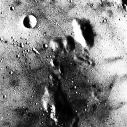 Histogram Equalization |
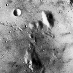 Histogram Optimization |
Here’s a common color test image:
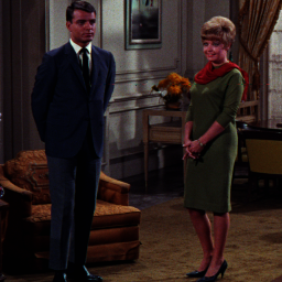 Original |
 Histogram Equalization |
 Histogram Optimization |
I’m quite pleased with my new algorithm but it’s not revolutionary. There are far better image contrast enhancement algorithms such as those that use Retinex theory:
https://ieeexplore.ieee.org/document/8500743
So why was I inspired to write a Glibs article? I was searching my computer’s hard disk drive for test images when I encountered one I couldn’t resist. I optimized its histogram and was surprised at the result which I reproduce here:
 Original |
 Histogram Optimization |
There’s practically no difference so I am forced to conclude that Lobster Girl is already optimal.
Footnotes:
[1] Remember them? They’re still in business as Edmund Optics but they don’t sell consumer/educational stuff anymore.
[2] Girls? What are girls? It was a few years after graduation that I belatedly realized there were girls at my high school.[7]
[3] 25MHz 386SL (low power SX) CPU with the optional 387SL FPU and 8MB of RAM! Power!
[4] I never said there would be no math.
[5] That wasn’t so bad, was it?
[6] I doubt that my new algorithm is original but I haven’t found references to anything similar, not that I’ve looked very hard.
[7] And then I was in an engineering school with an 8:1 male:female ratio.
Yes, image processing is one of my hobbies but I swear I can give it up any time I want.
🙂
There’s practically no difference so I am forced to conclude that Lobster Girl is already optimal.
🙂
Seconded.
Most color images are represented as three “monochrome” images for the red, green, and blue primary colors.
Except for the CMYK images. And as a movie buff, don’t get me started on two-strip Technicolor.
/sarcasm
Images are captured in RGB. Images are displayed in RBG on phones, computers, TVs, projectors, etc. Images are converted to CMYK for printing.
Printing is fantastically complex. Start with the reflective properties of the paper or target. Then the inks which even for a simple “good” printer are:
Cyan
Cyan (light)
Magenta
Magenta (light)
Yellow (so light that there isn’t usually a lighter ink)
Black
The math for reproducing accurate colors gets a little involved.
Back in my younger days, I was a printer. I did a short stint at a place that did four color separations for generating lithographic plates. The bulk of my time was spent burning and developing plates, but they did teach me how to do four color separations (film based). The first laser scanners were just hitting the market (insanely expensive). But even the old geezers knew their jobs were dead.
I mean, if nobody is gonna:
Enhance
Nice.
Also appropriate
There’s a first time for everything. Great song.
Concur.
Also I always pronounce the name Nikon in the bastardized English way. Who wants to be like that guy that says foreign city names in the local language.
Correct would sound like “nee + cone”. People would look at you like WTF?
Also kicked over to 50 Ways… which I haven’t heard in years.
Good one.
Why not enhance.
My link is an homage to that…
Yup, felt like we needed the original.
After that it’s been beat to death in “serious” shows. Notably spy and crime stuff where they pick a mole off a Polaroid.
I think the enlargement goes all the way back at least to Call Northside 777, where reporter James Stewart has a newspaper photograph blown up beyond all possible proportion to try to discern the date on a newspaper someone in the picture is holding.
It’s a big plot hole in an otherwise excellent movie.
You are right. The old fashioned photo enlargement was also a Hollywood staple.
https://vimeo.com/18748354
The Lobster Girl images are subtly different. The halo above LG’s sunglasses is brighter for example. I was previewing this article at the end of a long day, my eyes crossed, and the images formed into something that was practically stereoscopic. Yes! Ladies (If your appreciate such things.) and gentlemen, 3D Lobster Girl!
There’s practically no difference so I am forced to conclude that Lobster Girl is already optimal.
Has anyone ever identified Lobster Girl? I hope she is well.
Great article, Richard. I read the whole thing, but the pics made the most sense to me.
Thanks, brother!
Both Histogram Equalization and Histogram Optimization can produce horrible results. For some reason the examples in this article make the former look bad and the latter look good. The reason why is a mystery.
Thanks Richard, you lost me when you hadn’t discovered girls ’til way late in life. Those that know me IRL know that my glasses are really thick, it takes a whole lot of enhancement for me to see any difference. Also the math didn’t help either.
If Older Richard invented a Time Travel machine and went back to Younger Richard to inform him, “Dude, she’s so into you.”, Younger Richard wouldn’t have paid any attention.
I appreciate that there are folks interested in the low-level stuff like this – I never was.
I write software many levels higher than the true nerds who are into shit like operating systems and files and file processing.
OT. They are following you!
NYC paves way for homeless to move upstate — after some towns refused to take migrants
OMFG LOL.
Bring it on. Even my lib town is gonna go MAGA if NYC sends us a bunch of bums.
Most of the rest of the state is going to revolt bigly.
I have a vague memory that someone identified Lobster Girl.
A Colombian model if I remember correctly?
It’s been a while but you’d think that is something I’d remember.
You could never enhance the quality of a photo of a First. Even the attempt would lose what part of the essence of the First a mere camera could even capture.
I used to take some sports photos and owned an 18% gray card for setting white balance. But I never got this deep into processing. The histogram optimization of the color test image is nice. I got approved to shoot for MaxPreps but never sold much because I’m nobody’s idea of a salesman.
Not sure what was put out here. Civil Engineer.
Lobster Girl is an unalloyed good,
Do not understand all the pixel things.
Lobster Girl.
Let’s stop right there.
That’s not a limerick or a haiku.
Deal with it
If I ever invent a time machine, killing baby Hitler probably won’t crack my top 20, but killing whoever the fuck invented that trap snare that’s been ass-raping pop music for the last 15 years will be in my top 3.
Fucking heinous.
Right?! I just YouTube searched, that was on top, listened to like 3.5 seconds and said, “yup. That is Ted’s worthy” lol
JHTFC.
Oooh, I kinda like it.
Teds first (ha!) experience with Beat poetry.
Hunter Biden is suing Rudy Guiliani over the laptop. He continues to be coy about the laptop. It either exists or it doesn’t, depending on which day it is and which story he wants to tell:
I’d think step one is going to be a tough task and that’s proving that the device was stolen. And I can’t imagine anyone in the Biden White House is on board with this beyond his senile father. You are keeping the laptop in the news cycle. You are also putting the information itself on trial by claiming it was “manipulated.” Do you really want a court of law ruling on the validity of the information?
And what is there to gain? This is the sort of move an impulsive crackhead would make.
https://www.foxnews.com/politics/hunter-biden-sues-rudy-giuliani-laptop-accuses-ex-trump-lawyerhacking
I don’t understand their end game. Hunter will have to respond to discovery. He will be be asked if that was his laptop and if the emails, pictures, videos, etc are his. How does any of that help him.
The end game is you.don’t.fuck.with.the.Bidens. It’s about rubbing your nose in their lie’s while they laugh at you and get away with it.
I don’t think it will play out that way in a civil lawsuit. Hunter is also opening himself up to questioning about some of the same topics for which he is being criminally prosecuted.
It’s a dumb move all around unless you actually have truth on your side. Which he doesn’t.
I think he’s back on the crack.
This time they got him!
https://apnews.com/article/donald-trump-letitia-james-fraud-lawsuit-1569245a9284427117b8d3ba5da74249
But this totally isn’t politically motivated or anything…
Definitely not a judge playing it up for the media.
And statute of limitations? Don’t apply to Trump and we’ve seen that at least three times now.
Wasn’t the central argument here over how Trump was assessing the sizes of his properties? I’m glad the state is here to step in and protect large banks and lenders who were so grossly deceived by Trump’s dastardly overestimation of the size of his own apartment. None of those lenders, by the way, initiated any form of complaint. WE have a case of fraud where there is no party claiming to be defrauded besides the state which had nothing whatsoever to do with the deals.
It’s also funny how novel legal theories continue to be employed against Trump.
Ah, how we are shown that Trump was such a danger to democracy, mostly by Dems freaking out and changing laws willy. nilly.
When I was at Honey Harvest™ I was the lucky recipient of some maple syrup from Vermont. Thanks, Richard!
As was I! What MikeS said!
(Mike – STEVE SMITH has yet to be surreptitiously delivered to our neighbor’s patio. Waiting for just the right moment…)
STEVE SMITH KNOW HOW BE SURREPTI…SURPETI…SPURPIT…SNEAKY. BY SNEAKY, MEAN…
You’re welcome. There’s lots more there were that come from. I live where Maple Syrup is produced.
I got one too. Thanks so much.
Alright, we’re doing euphemisms.
I’ll watch almost anything Gordon Ramsey and he’s doing another season of “Kitchen Nightmares” where he supposedly rescues horrible restaurants. The new episode is a diner in Astoria, Queens that I’d been to a zillion times in an earlier life because I lived a couple blocks away for years. This should be interesting.
“This basement looks like a scene out of Saw.” LOL
Hah, my wife and I watch a lot of the G Man. The winner of the recently completed United Tastes of America is from right here in central Iowa. The first nightmare was a real disaster.
The food there was great 20 years ago. These two mooks running the joint were probably toddlers the last time I was there.
Coq au vin at a diner, lol.
One of Ramsey’s big things I totally agree with – Keep It Simple Stupid.
If you’ve not seen the OG British version of that show, it’s worth tracking down some episodes. He does the voiceovers and he is also way, way less shouty in general. He just comes across as genuinely concerned and wanting to help people get their shit together.
Much superior to the Fox version.
I’ve seen some of his British shows.
I like both approaches.
He’s descended into self-parody these days. His earlier British series were great. Ramsay’s Boiling Point captures him when he was still a brash actual chef and not yet an international TV star. Good little docuseries.
I was in the latter stages of high school before I found out the really cool space pics from Hubble that I’d been using as desktop wallpapers were phony as a 3 dollar bill. My disappointment was only partially mitigated by my newfound ability to ruin it for everyone else, too.
This article’s featured image:
https://www.glibertarians.com/wp-admin/upload.php?item=116167
Was the best I could do with the computer I had at the time. I was trying to mathematically accurate colors.
As a layman, it looks remarkably good, IMO. All the more so considering when it was taken and the equipment with which it was processed. I would have bought that it was a recent Hubble image.
So, my doctor has suggested that I poop in a box and send it away.
Glib thoughts?
Any destination in particular, or just some random citizen?
You could be the lucky winner.
FIT test? Certainly more pleasant than the full colonoscopy, but it’s limited in scope and does have false negatives. If you have a family history of colon cancer, it might be better to just bite the bullet and learn the wonders of “twilight sleep.”
Apropos:
https://www.youtube.com/watch?v=waRoEw0P1og
Cologuard?
My favorite part is that the instructions say “Don’t drink the preservative liquid”. Which leads me to believe some lawyer put that in after some asshole drank the preservative liquid.
I got one of those last year. Then forgot about it in my closet. But it doesn’t expire until February so I’ll do it before then.
As Pat said, this is for people without a history of cancer. My family has plenty of heart disease and high blood pressure, but very little cancer and no colon cancer, so my Dr. recommended the box.
Hopefully you didn’t forget about it after filling the box.
They suggest that if they think you’re low risk for colon cancer, but it’s time for you to get a colonoscopy.
I am on the every-3-years colonoscopy schedule because the last time, they found precancerous polyps.
Better to send it away. It’s painless. I think it’s sort of a test.
“Well, the results are inconclusive, I think you should have a sigmoid (sort of a beginner’s colonoscopy).”
Then comes “You know, it wouldn’t hurt for you to have a colonoscopy”
When you reach 75 you can stop, if the results have been negative all along.
Go for it. Ramming a tube up your bunghole seems like a step backward.
I did the Cologuard thing. Not covered by insurance.
My best friend had his entire colon removed at 26. He’s still kicking. Colostomy not withstanding.
Colon cancer is not a joke, but I don’t think a colonoscopy is the only way to check on it.
YMMV.
Ugh I had that for a few months in 2020.
I want to know why, if we’re so smart, we can’t just wave a hypospray and solve all our medical problems by now. McCoy was right – our medicine is still so barbaric.
Money is the answer. As always.
G-d I love that show.
I mean, I’d send it away. If you want to keep it I guess it’s your call. I just don’t think that would be very helpful.
No kink shaming.
“Remember them? They’re still in business as Edmund Optics but they don’t sell consumer/educational stuff anymore.”
I do.
Today I made split pea soup. It was on very low. It wasn’t even boiling. I left for around 45 minutes or so.
I come back, and the living room is filled with smoke. My first reaction was to ask my mom why she didn’t say anything about the smoke. She says she didn’t notice. I’m not happy with this answer.
I go into the kitchen. The cover was ajar (I’m guessing steam or hot air knocked it out of place) with smoke pouring out of the pot. The burner was glowing bright red. I turned it off and put the pot in the sink. Then I opened all the windows.
Upon further inspection there was about an inch of charcoal in the bottom of the pot.
Fortunately, the kitchen didn’t catch fire.
This is the third time recently that something burned or nearly burned on that burner. Which never happened before. So I think I need a new stove.
Creepy. You might just replace it. Not worth a risk. You could try just replacing the knob and regulator. It might have gotten liquid in it and started shorting.
“You could try just replacing the knob and regulator.”
Yes, that could be it. The other day I turned it down, and it responded by glowing hotter. So it seems broken.
I think I was more upset about my mom’s lack of reaction.
How old is she?
She is very old, and has been diagnosed with “mild dementia”.
Yeah, one of the signs my dad was going that way was when he tried to pour hot oil into a plastic milk jug. It is a hard row to head down.
Yup, I’d say it’s the control unit for that burner. Hopefully they are separate mechanical controls and it doesn’t take a whole new control board or something.
I agree. It’s nine years old. So I’m thinking of replacing the whole thing.
Probably not a bad idea. We did the same when the same thing happened to us. I was in favor of just fixing it, but I was outvoted 0-1.
I spent a few weeks fixing up our old dishwasher, but so much was worn out with it by that point it was a fools errand. You would get minor improvements, but it needed everything done in the end. Home Despot had a sale, and bobs your uncle. I even had them install it (free), on Valentines day (winning!)
So, I’m wondering. Could your mom have turned the heat up?
I looked at the knob and it was where I left it.
Okay, good.
She wouldn’t interfere with my cooking. I’m not worried about that.
It was more like she didn’t understand why I was upset, and said she didn’t say anything because she didn’t want to make me more upset?
Well, I inderstand your concern, but maybe she just really didn’t notice the smoke? I got a water delivery one day and my delivery dude said, “You need to get out now, You’ve got a gas leak.” I never smelled the sulfur. However, I DO have anosmia and often smell things that aren’t there or don’t smell things that are. I had to throw out a whole bottle of perfume because one day I woke up and it just smelled like cat pee.
So, like, with dementia, sensory issues can go along with.
I am 59 and a voracious reader. Scored perfect in reading comprehension on the ACT test back in the day.
I have never encountered the word “anosmia” before.
I truly want to thank you for educating me today.
I smelled it multiple times in the last couple years at my last place, and the friendly maintenance man who literally spoke not a single word of English disagreed.
For that reason – and that reason only – I’m sort of pleased with the electric range I have now.
“Well, I inderstand your concern, but maybe she just really didn’t notice the smoke?”
Sorry, for not being clear. I didn’t mean saying something about the smoke, but after I came back and explained what happened. She said he didn’t say anything because she didn’t want to make me more upset. Which I found more upsetting.
@milo, you’re welcome! I wouldn’t feel bad, though, because medicine is like its own language.
I ALSO have phantosmia. My most common phantom smell is stale cigarette smoke.
When I had my daughter, it jacked up my sense of smell for 5 years. It never really went back right, and now it’s fluctuating on me again.
@Count, sorry. I think it was I who misunderstood. Yes, that would be upsetting.
Good Lord! Learned another word. Phantosmia.
Keep them coming, as I am too old and tired to discover the infinity that I do not know.
Sony has apparently been hacked once again.
We won’t be getting leaks this time, apparently. They are threatening to sell whatever data they may or may not have obtained.
There is no such thing as “batten down the hatches” and the sooner the world understands that, the better.
All your base are belong to us – time to start behaving as if you know that fact.
Good morning peeps.
🌄🐥
Love song Wednesday again:
https://m.youtube.com/watch?v=3zQWWjoYrzA
🎶🎶
I like this version.
Good morning all!
Hadn’t been my plan (plan? what plan?) but here’s something extracted from Einstein on the Beach, the first of Glass’s operas. We’ve now hit something from each of the ‘Portrait Operas’, albeit in reverse order.
Violin Solo Music from Einstein on the Beach
Share and enjoy!
Good morning, Beau, Sean, U, Stinky, and Roat!
My boss is working from home again today (workers coming to finish a bathroom remodel job,) and HIS boss is supposed to have a golf outing. It’s certainly warm enough for golf, but it might get a bit wet, so we’ll see how bossless we are at the office today.
https://www.cbsnews.com/philadelphia/news/center-city-stores-ransacked-looted/
🙄
Shoot to Kill.
“Our cameras also saw looting at the nearby Lululemon store on Walnut Street in Rittenhouse Square.”
Seems like they’d steer clear of Rittenhouse Square.
Is there a lucrative black market for yoga pants? 😕
LOL, that is too much. Rittenhouse Square is named after this white supremacist:
https://en.m.wikipedia.org/wiki/David_Rittenhouse
I expect a name change in short order.
“Have you voted for a Democrat in the last ten years?”
Mornin’, reprobates! Definite chill in the air, autumn is here.
Good morning, ‘patzie! Come to SW OH – after a couple of days of damp/low 70s, we’ll be sunny and back up in the upper 70s/low 80s for several days! 😃🌞😎
48 here, should break 60 later. There is that weird yellow ball in the sky again, hasn’t been around for a week.
Mind the radiation, though it’s relatively mild. Your handsome hat should offer some protection.
The hat helps, but house arrest is the winner. I’m comfortable as long as I am seated, walking around is problematic.
I wish you all the best. As long as you can at least sit comfortably life is good.
It has been pleasant. I’ve been leaving windows and the back door open this week. The forecast for the state fair visit is good. I love autumn.
If you’re going to the state fair, it might as well be spring.
https://m.youtube.com/watch?v=TXMEVTtAZkI
Light windbreaker kind of day.
And I drove the GTI to work…wheeeee!
Kleine GTI?
https://m.youtube.com/watch?v=3zcm4oS9IaM
At no time this morning did I get airborne. I swear.